Prologue: Film Fan is your very own personalised film recommendation engine. Please check it out here: filmfan.ai. A full walkthrough of the site’s features and inspiration is covered in a previous post: here. This is a 5 part series to break down how I designed and built Film Fan, from all angles: data, engineering, analysis, machine learning, speed, productionisation, cost etc. For reference, please also see the previous posts in this series:
- Film Fan – Under the hood – Overview
- Film Fan – Under the hood – Data
- Film Fan – Under the hood – Data Collection
This post is dedicated to arguably the sexiest but most enigmatic aspect of a data project – machine learning (a core part of an AI system). We discuss the types of machine learning approaches explored and how the final model was optimised. Finally, we cover how the solution was developed and deployed to a production grade system for an enduring benefit.
Goals
Recapping Film Fan’s goals stated in the overview, “I just wanted an easy way to find films that would have a ‘life-altering’ impact on me.” Another way of thinking about this is like a search engine, of the ~20k films in the film universe, which of those are most likely above a certain personal quality threshold – i.e. are ‘life-altering’ or ‘Awesome’ for me.
A data project at its core is an optimisation project, hence the goals are necessarily quantitative. So then how do we define a metric against which to measure the success of the project? Well, we could just say how many films have been recommended, but then if we’re only just optimising for this, the quality of those recommendations could be too low. So then we also need to ensure quality recommendations. These two metrics in machine learning are formally defined as the following counts as proportions of the total recommendations:
- Precision: how many recommendations are actually correct (i.e are an actual ‘life-altering’ film)?
- Recall: how many of the ‘life-altering’ recommendations that theoretically exist for this user have been found?
There is naturally a trade-off between these two because over optimising for one can de-optimise the other. Hence if we want to have a balanced view of precision and recall, we use F1 score = 2 x (Precision x Recall) / (Precision + Recall). All models assessed and tuned for Film Fan were optimised in this manner. Another metric during the tuning process was AUC which is when you want to understand the model’s performance over all possible thresholds (the specific value that determines the cutoff point at which predicted probabilities are converted into class labels), making it suitable for tasks with imbalanced data or when ranking predictions is important like Film Fan (most films you review you haven’t even watched let alone will rate as ‘Awesome’).
Here are some examples of Awesome films I’m trying to find:
Selecting a state-of-the-art model
In order to have a quality solution, the machine learning model selected must be state-of-the-art, it also needs to be adequately tuned on your data- these are just prerequisites. Once this is achieved, it’s about feeding the model more and higher quality data to extract the maximum value from that data. Film Fan is a content based recommender, which is a classification problem. After researching online and speaking to the best industry experts, the best models for this scale of data problem were found to be: Gradient Boosting Machines (GBM). Deep learning is another option but more complex to build while not materially better than GBMs; hence a little heavy handed for the task at hand.
How to interpret decision tree models
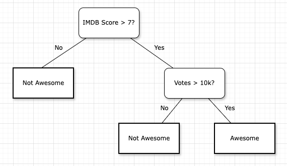
The final machine learning model selected was the popular GBM library called XGBoost. Another similar but less performant model Random Forest (see below “…data features…”) was also used to explore the data. In order to interpret these models, we can think in terms of their building blocks, which are decision trees. Let’s start with an example basic decision tree from our data below:
Following this tree example, we can see that if a film has an IMDB Score > 7 and (number of) votes > 10k, then it’s classified as ‘Awesome’, otherwise it is ‘Not Awesome’. This is a very basic case however. Now let’s improve it step by step…
Improvement 1: Build full sized decision tree
Use all ~100 data features (i.e. calculated columns) to create a decision tree with all nodes and optimised thresholds (i.e. yes/no cut-off points).
Improvement 2: Build many full sized decision trees (Random Forest)
Instead of 1 tree, build 100s or 1000s of independent trees in parallel and combine the results. Each tree is generated by randomly selecting data points with replacement, so some data points may appear multiple times, while others may be omitted.
Improvement 3: Build many full sized decision trees that get better each time (XGBoost)
Rather than building trees independently, build sequentially and focus on correcting errors from previous trees. This results in the last tree generated typically with higher prediction accuracy.
The data features which feed the model
As mentioned in the data post of this blog series, the data used for machine learning, i.e. the features in this content based classifier are all based from the fields you would see in an IMDB film page: Score, IMDB Rating, Directors, Actors etc…
We take these raw values and transform them into data features for the machine learning training data. For example:
Raw column:
- cast: “Brad Pitt, Matt Damon”
Training columns:
- cast0: “Brad Pitt”
- cast1: “Matt Damon”
As mentioned in previous posts, the features can be preprocessed in advance (outside of the training and scoring of the machine learning for each user) since they are purely linked to the film itself (i.e the nature of a content based recommender). Within this preprocessing we must deal with missing or incomplete data in the following ways:
- Features that are missing a value – use the mode (most common value for that feature) – (e.g. bw or colour, use colour)
- Features that exist in too few films, simply delete (e.g. cinematographer #6)
- Missing continuous columns (median budget in 1999 was 10M, use this value if film doesn’t have budget)
Importance of each feature in machine learning
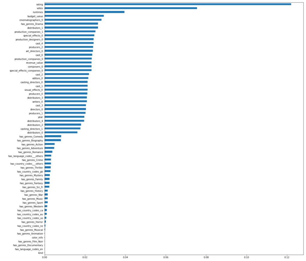
During the building of a machine learning model, we can take a look at which features are most important for each user: using sci-kit-learn’s (Python library for machine learning) feature importance functionality. “User A” example shows that not surprisingly the IMDB Rating, (number of) votes and the runtime are the most important features to find the ‘Awesome’ films. However, for another user (“User B”- who had reviewed much fewer films), the: visual effects, cinematographer and production companies were most important for finding an ‘Awesome’ film for them. This gives some confidence that individual user recommendations are worth the effort since taste and hence the way features are used by the ML model can vary widely between users.
Feature importance for User A

Feature importance for User B
Tuning the model and results
From a system point of view, tuning a model simply means – “What settings are needed on this machine to make it work most optimally in this environment?”. In a machine learning context these settings are referred to as hyperparameters which change depending on the model. This is analogous to tuning the engine in a car, where you want the car to run most optimally (in terms of power/efficiency etc) by modifying the settings (e.g. air-fuel ratio, ignition timing etc).
The tuning process for all classification models like this involves “Cross validation” to find the best hyperparameters, which was the same approach for Film Fan. Cross validation involved partitioning(splitting) the training data (i.e. set of film attributes and their reviews) into a random 80% of the data to train the model, then the remaining 20% to test the model – to find out “how well did the model perform on unseen data?”. Then we do this process hundreds of times with a variety of different hyperparameters to determine the best values to use. Also instead of simply splitting the data once 80/20%, you split perhaps several times (depending on the size of your data).
The hyperparameters to tune for XGBoost are:
- scale_pos_weight: A parameter used to control the balance of positive and negative weights, particularly useful in imbalanced data like Film Fan. It is the ratio of the number of negative class samples to the number of positive class samples (‘Awesome’ films).
For Cross Validation – these parameters are set to ensure the cross validation process is fair
- n_splits = the number of partitions into which the dataset is divided.
- n_repeats = the number of times the cross-validation process n_splits is repeated (i.e. repeated with a different random set of data in that partition).
Here are the results of this process using training data for my own user data:
Observing the above, we note:
- scale_pos_weight can affect the model performance: AUC (test_roc_auc), precision and recall. Setting this appropriately for all users is important. What works for one user may not work as well for another – depending on how imbalanced their training data is.
- The n_splits and n_repeats parameters were set to 3 and 5 respectively as it was observed that changing them had negligible effect on the outcome, so these nominal values were used.
- For the top results settings, even though the AUC doesn’t change materially, the precision and recall can vary considerably.
- After experimentations like this for various users’ data, the scale_pos_weight was set to 1 to optimise the quality of the recommendations, considering also the machine learning job which uses a weighted average (see below).
Comparison to off-the-shelf machine learning
The results from these experiments were also compared with an off the shelf machine learning tool called Auto ML Tables from Google (now rebranded Vertex AI). This tool and similar off-the-shelf tools run a variety of different models against your training data to find the best possible predictions. In this case, it did not perform materially better or worse than the above results. These automated tools can save you time during development however charge considerably more than a simple cloud compute job to train a model. Here’s a rough comparison at the time of experimentation (in AUD):
- Train model using Auto ML Tables: $20/hour
- Train custom model using Cloud Run: $0.10/hour
$20/hour might not seem like alot but it does add up when you run training jobs for many users, every 30 mins(like Film Fan).
It does take time and specialist skills to build a model, however once it’s built, the maintenance and complexity is much lower than most other parts of your ecosystem. For example, the model training code for Film Fan is simply 1 module of roughly 100 lines of code. It’s been running in production without fault for over a year.
The productionised training job for the model
Once we have selected and tuned the model, the next step is to systematise this task in an automated data processing job. As mentioned in “…jobs…” of overview page (see “Users and recommendations” job), from a system point of view, this is just another data processing job – using Cloud Run. Although it does have machine learning training, the pre-processing happens separately within the job “Process film data”.
Here’s a rundown of the main steps in the machine learning component of the ‘Users and recommendations’ job:
- For every user that has added more reviews since the last job:
- Train and score a model for ‘Watched’ – predicting films that the user would review as ‘Awesome’ under ‘Watched?’ flag on review screen.
- Train and score a model for ‘Would watch’ – predicting films that the user would review as ‘Definitely’ under ‘Would watch?’ flag on review screen.
- Apply a weighted average to the above two scores for all films.
- Filter for only those films above a threshold to be classified as ‘Awesome’ – these are the users’ recommendations.
- Rank and sort the recommendations by score (highest at the top).
- Store in Google Cloud Storage, Firebase and BigQuery (see previous posts in this series to know how each storage is used)
For better accuracy in the training of models, a one-vs-rest classifier was used to ensure that the model is not just predicting ‘Awesome’ films, but predicting what classification overall applies for each film (e.g. ‘Terrible’, ‘Bad’, ‘Good’, ‘Awesome’).
Model reproducibility
Each time a model is trained, it can be reproduced in the future since the following data is always captured:
- The job ID that trained the model, which has:
- Timestamp
- Hyperparameters
- User ID
- All of the recommendations and scores/ranks as outputs to that job ID.
- Also all reviews from the user and their historical states are always captured (since they could change their review)
Given this and using the committed code in GitHub, we can always reproduce a model for a given user at any point in time. This is helpful not just for auditing purposes but also for analysing how well your model has improved over time.
Results and challenges
Here are some wonderful film recommendations, I’m looking forward to watching!
Let us know how our recommendations are for you!
And finally, it’s worth noting that besides the technical and analytical challenges in creating these recommendations, there are other data challenges at a human level:
- We need enough reviews! – It’s hard to know exact numbers, but perhaps 10 watched and 10 unwatched film reviews would be a minimum for this to work. Ideally 100+ of each, but the more the merrier (I’ve done nearly 12k reviews). My own personal recommendations have improved the more I’ve added and updated my reviews over time.
- Getting objective reviews – sometimes I look back at old reviews and realise at the time I probably wasn’t being objective enough and just reviewing for speed instead of accuracy (there’s a balance to be had).
- Changing mood – Being in a good or bad mood could affect how likely you are to give positive or negative reviews.
- Changes over time – My taste certainly changes over time. For example, I’m no longer interested in Disney movies as much as when I was a kid. Maybe even in 5 years, taste could also change from now.
- Sometimes the recommendation is off – this is the nature of machine learning, it’s merely the best possible prediction based on the data (it’s not fact). But it’s okay because when I change the review, the model will retrain and produce better recommendations, “the machine learns”


